Developing a bioformulation stability profile

Executive Summary:

When used in combination, light scattering and microcapillary viscometry can be used to develop a stability profile to screen biotherapeutic candidates, with light scattering providing a suite of dilute solution properties and microcapillary viscometry providing analysis of viscosity even at high sample concentration. The ability to handle both low sample volumes and high sample concentrations makes these two technologies ideal for moving the biotherapeutic screening process, both in terms of prediction and confirmation, to earlier points in the development pipeline.

Here we describe the development of a bioformulation stability profile, derived from sub-micron light scattering analysis and microcapillary viscometry.

Introduction

Light scattering is a staple technology within the biopharmaceutical industry, routinely used to screen biotherapeutic candidates and formulations. Historically, submicron light scattering technologies, e.g. static (SLS), dynamic (DLS), and electrophoretic (ELS) light scattering, have primarily occupied a monitoring role within formulation development, with classic examples being the use of DLS to test for the appearance of aggregates during stress testing, or the use of ELS to monitor changes in the sample’s zeta potential and subsequent colloidal stability with environmental changes such as pH and ionic strength. Malvern Instruments’ Zetasizer Nano system combines all three light scattering technologies, and is able to provide information on the particle size distribution, polydispersity trend and interaction parameter from DLS, the 2^nd virial coefficient from SLS, and the electrophoretic mobility and effective charge from ELS. Each of these properties, measured under dilute conditions, has been found to be empirically “predictive” of aggregation propensity, solubility, and increased viscosity, under the high concentration conditions typical of biotherapeutic formulations.

While predictive parameters are beneficial for purposes of screening out candidates likely to be problematic, candidates that pass the screen must eventually be tested for stability and viscosity under the high concentration conditions expected for the final bioformulations. Historically, viscosity testing has been delayed until the later phases of the formulation development, due to sample volume limitations. However, microcapillary viscometry provides a way to eliminate this hurdle. This technology, embodied within Malvern Instruments’ Viscosizer 200, combines UV area imaging with dual-pass microcapillary detection to measure the viscosities of high concentration biotherapeutic formulations using as little as 10 µL sample volume.

By coupling the parameters obtained from light scattering with those obtained from microcapillary viscometry, a comprehensive bioformulation stability profile may be derived for protein therapeutic candidates, for use during early formulation development screening. In addition to the obvious time and resource savings associated with reducing the size of the candidate pool earlier in the development pipeline, the stability profile gives the formulator the potential to improve product performance, while simultaneously providing insight into the mechanisms associated with formulation instability.

Biotherapeutic Screening Parameters

Analytical instrumentation can be used to both monitor and predict sample properties. An example of monitoring using static light scattering, for instance, would be the determination of molecular weight and degree of conjugation for the purpose of determining the number of glycosylation sites on a mAb. Light scattering techniques are routinely used to monitor a variety of properties during bioformulation stress testing, to check for the presence of aggregates or sub-micron particles. Alternatively, a formulation property measured under one set of conditions can be used to predict the behavior of the formulation under a different set of conditions. An example of this capability is the screening of biotherapeutic candidates for their aggregation propensity at high concentrations (those typical of formulation conditions) based on 2^nd virial coefficient values measured under dilute solution conditions. In addition to the 2^nd virial coefficient, other light scattering properties being integrated into screening assays include size distribution and polydispersity trends, the DLS interaction parameter, and effective protein charge.

Size Distribution

Dynamic light scattering (DLS) is a low resolution technique, requiring a 3x difference in size in order to achieve baseline resolution in the particle size distribution (PSD). The scattering intensity, however, varies with the 6th power of the hydrodynamic radius. So while DLS cannot resolve protein oligomers, its high sensitivity to larger particles can be exploited to monitor subtle changes in the distribution of protein oligomers. Consider for example, the DLS size distributions shown in Figure 1 for IgG diluted in two buffers, where R_S is the Stokes radius measured in the limit of infinite dilution. As the concentration is increased, buffer 1 (left) shows an increase in the width of the distribution, suggesting the formation of oligomeric species with increasing sample concentration. These results are indicative of reversible self-association. For buffer 2 (right), however, an increase in sample concentration leads to an apparent downward shift in the size distribution, with no significant change in the distribution width. These results are indicative of electrostatic repulsion, with the apparent decrease in size being attributable rather to an electrostatically driven increase in the diffusion coefficient.

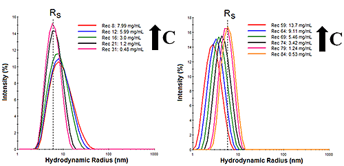
Figure 1: Concentration dependent size distributions for IgG in buffer 1 (left), with Tween stabilizer, and buffer 2 (right) with aspartic acid stabilizer.

Polydispersity Trend

The mechanistic interpretation of the results in Figure 1, e.g. reversible self-association vs. electrostatic repulsion, is a little easier to visualize when the results are presented in the graphical format shown in Figure 2. The DLS polydispersity (Pd) is the width or standard deviation of the size distribution, and is represented by error bars in the concentration trends shown below. As noted in this figure, both the mean size and width of the IgG oligomeric distribution decrease with decreasing concentration in buffer 1, indicative of reversible self-association. For buffer 2 though, the width of the distribution is independent of sample concentration, i.e. remains constant, but the mean size at higher concentrations is “smaller” than R_S. As R_S is defined as the physical size of the antibody in the absence of restricted diffusion (viscosity) or particle interaction effects, the only explanation for a protein to appear smaller than it actually is, is if the particles are moving faster than the diffusion velocity. In the absence of a temperature increase, electrostatic repulsion is the only force available to increase the diffusion velocity.

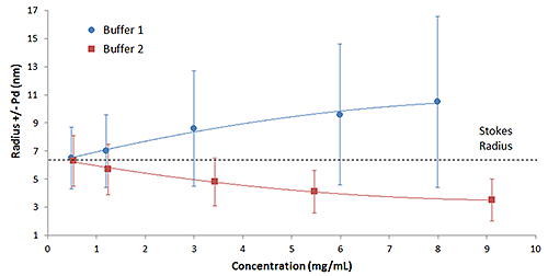
Figure 2: Mean size and polydispersity trend with concentration for IgG in buffer 1 and buffer 2, with the polydispersity represented by error bars.

DLS Interaction Parameter

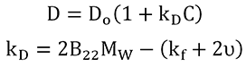
The qualitative information contained within the size distribution and Pd trend can be quantitatively expressed with the DLS interaction parameter (k_D). k_D is extracted from the slope of the concentration dependence of the mutual diffusion coefficient (D) as indicated in the expression shown below, where D₀ is the self-diffusion coefficient in the limit of zero concentration (C) from which the Stokes radius is derived, B₂₂ is the 2^nd virial coefficient, M_W is the molecular weight, k_f is the 1^st order concentration coefficient of the friction coefficient, and υ is the partial specific volume.

Empirically, k_D has been shown to be correlated with both aggregation rate and formulation viscosity. Samples exhibiting larger positive k_D values exhibit a lower propensity for self-association and aggregation, as well as lower viscosities at the high concentrations typical of biotherapeutic formulations. Based upon these empirical predictions, it would be expected that buffer 1 from the earlier example, which exhibited reversible self-association, would have a smaller k_D value in comparison to buffer 2, which exhibited stabilizing electrostatic repulsion. Figure 3, which shows the concentration dependence of the diffusion coefficient for IgG in buffers 1 and 2, confirms that expectation.

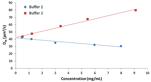
Figure 3: Concentration dependence of the measured diffusion coefficient for IgG in buffers 1 and 2.

Second Virial Coefficient

There are 2 components to k_D: a thermodynamic component (B₂₂M_W) and a hydrodynamic component (k_f + υ). The predictive power of k_D is a consequence of the thermodynamic component, specifically B₂₂. The 2^nd virial coefficient (B₂₂) is representative of the pair-wise interaction potential between like molecules. Positive B₂₂ values are indicative of highly solvated samples. Negative B₂₂ values, however, are indicative of samples with a propensity toward self-association and low solubility.

B₂₂ is extracted from the slope of a Debye plot, which is representative of the concentration dependence of the sample scattering intensity, as indicated in the expression shown below, where K is an optical constant, R

θ

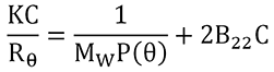
Figure 4 shows a comparison of the Debye plots for the previous IgG in buffer 1 and 2 example, along with a 3^rd buffer utilizing a lactose stabilizer. As seen in this figure, buffer 2 and 3 both exhibit positive virial coefficient values, with buffer 1 exhibiting a negative virial coefficient. Based upon empirical predictions then, buffer 2 would be expected to be the most stable and buffer 1 the least stable, with buffer 3 somewhere in between.

Buffer 3 highlights the importance of the hydrodynamic component in k_D. While not shown in Figure 3, IgG in buffer 3 exhibited a k_D value that was more negative than both buffers 1 and 2, with measured k_D values of 31.9 mL/g, -5.2 mL/g, and -9.7 mL/g for buffers 2, 1, and 3 respectively. If the hydrodynamic component were ignored, it might be erroneously concluded that buffer 1 is likely to be more stable than buffer 3 - This is disproved by the B₂₂ results. It is for this reason, that k_D, while easier to measure than B₂₂, is generally restricted to use as a stability predictor within the k_D > 0 region, with B₂₂ considered the more reliable predictor across the widest range of formulation conditions.

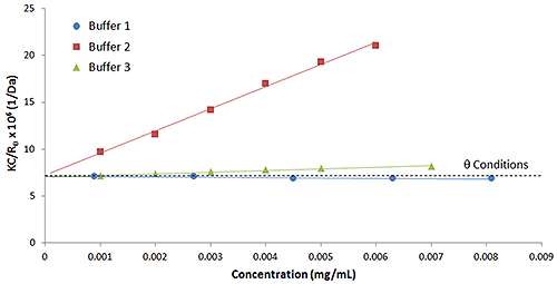
Figure 4: Debye plots for IgG in buffers 1, 2, and 3, with theta conditions at B₂₂ = 0 represented by the dashed line.

Intrinsic Properties

Here, we define “intrinsic” to identify properties of the protein within the formulation buffer, but in the absence of concentration dependent effects that impact reported values. Concentration dependent effects include restricted diffusion and/or electrostatic interactions, and by determining intrinsic properties in the limit of infinite dilution, these can be minimized.

Oligomeric Molecular Weight

The weight averaged molecular weight (M_W) is derived during the course of an ensemble SLS 2^nd virial coefficient measurement. Because it is mass weighted, small amounts of oligomeric species can have a large effect on M_W. If the monomeric molecular weight is known, as it often is, then comparison to the oligomeric M_W gives one a qualitative idea of the degree of oligomerization.

Stokes Radius

The Stokes radius (R_S) is derived during the course of an ensemble DLS interaction parameter (k_D) measurement. The Stokes radius is an intensity weighted average size of the oligomeric distribution. Comparison of the Stokes radius to the known hydrodynamic size of the monomer gives one qualitative information regarding the oligomeric distribution in the absence of concentration dependent thermodynamic effects.

% Polydispersity

A third intrinsic property that can be used to provide qualitative information regarding the oligomeric distribution is the % polydispersity. This value is derived during the course of a DLS k_D measurement (%Pd = Pd/Size). While DLS cannot resolve oligomers, the width of the intensity weighted size peak is very sensitive to the presence of oligomeric species. The rule of thumb for monomeric protein samples is that %Pd should be less than 15-20%. A %Pd value greater than this is a clear indication of the presence of oligomeric components.

Ideally, M_W and R_S, along with the resolved oligomeric distribution and percent purity, would be measured via light scattering coupled to size exclusion chromatography (SEC-LS), and in practice, they often are. With that said, the data needed to generate these values is available (with no additional experiments) once the measurement of k_D and B₂₂ is performed. This, coupled with the absence of SEC column limitations, makes them useful parameters to determine and include in a stability profile.

Net Charge

The net charge (Z) is calculated from the electrophoretic mobility (µ_E), measured using ELS, and the Stokes radius (R_S), measured using DLS, as indicated in the expression shown below, where h is the viscosity, κ is the inverse Debye length, f(κR_S) is the Henry function, and Z_Eff is the effective charge at the slipping or interaction plane.

The net charge is the principal driver from the standpoint of colloidal stability. The greater the net charge, the greater the electrostatic repulsion between like particles. For antibodies and other proteins, the net charge is particularly important, due to the heterogeneity of the surface charge, which can lead to attractive dipole-dipole interactions at the higher concentrations typical of biotherapeutics. For antibodies exhibiting large dipole moments, the net charge must be large enough to counter these attractive interactions; otherwise, aggregation and increased viscosity at high sample concentration is probable. As a general rule of thumb, an effective charge of 4-6 is typically indicative of good colloidal stability for mAb formulations, with an effective charge > 6 being indicative of excellent stability.

The table below shows a comparison of the net and effective charges of the previous IgG in buffers 1, 2, and 3 as an example. These samples are ranked in order of decreasing stability, as predicted by the 2^nd virial coefficient. A 4th buffer, PBS with no stabilizer, noted as “#4”, is included for discussion purposes.

As seen in the table above, the effective charge predictions are generally consistent with the B₂₂ predictions, with only buffer 2, the sample exhibiting a large positive B₂₂, indicating good colloidal stability. At lower values however (buffers 1 and 4 for example), the charge is a less effective predictor, as dipole-dipole interactions become a factor in this realm. These dipole-dipole effects are accounted for in thermodynamic B₂₂ values, but not in net or effective charge values.

Melting and Aggregation Temperature

The protein aggregation onset temperature (T_onset) is the minimum temperature required to induce aggregation in a protein formulation. As a consequence of the R⁶ dependence of the scattering intensity, subtle changes in the aggregation state of a protein formulation are easily detected with light scattering techniques. Figure 5 shows the DLS thermal ramps for the previous IgG in buffers 1, 2, 3, and 4.

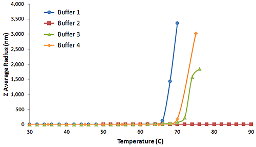
Figure 5: DLS thermal ramps for IgG in buffers 1, 2, 3, and 4, showing the sharp increase in the Z average size at T_onset, indicative of the onset of aggregation.

As evident in the above figure, aggregation leads to a sharp increase in the Z average size, clearly defining T_onset for IgG in buffers 1, 3, and 4. Buffer 2 however, shows no evidence of aggregation up to a temperature of 90°C.

The melting temperature (T_m) is the temperature at which protein unfolding occurs. T_m then is indicative of the inherent structural stability of the folded protein, and in the absence of denaturation, T_A would be indicative of the colloidal stability. With that said, T_onset tends to follow T_m, and is usually a direct consequence of the T_m denaturation, rather than a loss of colloidal stability. In fact, it’s only when T_onset precedes T_m that it can be used as a stability predictor, although the use of T_m as a predictor of inherent structural stability is routine within bioformulations.

The magnitude of light scattered from a sample is proportional to the square of the molecular weight and the square of the refractive index increment (dn/dC), which is proportional to the molecule density or the partial specific volume. As proteins unfold, they expand; which leads to an increase in size and a decrease in dn/dC. So light scattering can also be used to monitor thermal induced denaturation. Consider Figure 6 for example, which shows expanded views of the DLS thermal ramps for IgG in buffers 1 and 4, along with the simultaneously measured scattering intensity.

Figure 6: Expanded views of DLS thermal ramps for IgG in buffers 1 and 4, along with the simultaneously measured scattering intensity.

In buffer 1, a sharp increase in hydrodynamic size is observed at 66°C, indicative of thermal induced aggregation, i.e. T_onset. Prior to T_onset however, a small increase in size accompanied by a sharp decrease in scattering intensity is observed at 56°C. The small increase in size could be a result of either self-association or unfolding (either fully or partially). The decrease in scattering intensity, however, suggests a reduction in refractive index differential (dn/dC), which would be indicative of unfolding, with 56°C then being the T_M. In buffer 4, T_m and T_onset are reversed, with the small increase in size at 55°C being accompanied by an increase in scattering intensity. This increase suggests an increase in molecular weight, likely arising from thermally induced self-association prior to denaturation and subsequent agglomeration at the 70°C T_m. This early T_onset event, e.g. pre-T_m, is sometimes referred to as T_onset initial or even T_onset association, depending upon the research group, with the singular T_onset descriptor being reserved for the onset of gross agglomeration.

Viscosity

While the upper viscosity limits for biotherapeutic manufacturing and subcutaneous injection are company-dependent, typical values are considered to be around 20 cP and 10 cP for processing and subcutaneous (SubQ) injection respectively. At the high concentrations typical of antibody-based biotherapeutics, optimizing formulation conditions to not exceed these limits can be challenging. While the light scattering predictors discussed earlier can be helpful in screening out problematic candidates and formulation conditions, and even rank ordering successful candidates in terms of expected stability and manufacturability; ultimately, the formulation viscosity must be measured. Figure 7 shows the concentration dependence of the viscosity of IgG in buffers 1 and 2, measured using microcapillary viscometry. Consistent with the light scattering predictors, buffer 2 is the most stable, with SubQ and processing concentration limits of 148 mg/mL and 176 mg/mL respectively. In comparison, IgG in buffer 1 exhibits SubQ and processing concentration limits of 137 mg/mL and 153 mg/mL respectively.

Figure 7: Concentration dependence of viscosity of IgG in buffers 1 and 2, with dashed lines representing the SubQ and processing limits.

The Bioformulation Stability Profile

The stability profile of a biotherapeutic candidate is a collection of stability predictors and descriptors that provides insights into the developability and manufacturability of the bioformulation. The resultant stability profile for the IgG in buffers 1 and 2 examined in this report is shown below. The green, yellow, and red coding indicates “go”, “caution,” and “no go”, while “RSA” and “CR” represent reversible self-association and charge repulsion. While specific targets are dependent upon the company and screening program, the values indicated in this example are reasonably representative of typical target values. That said, the developability and manufacturability conclusions are somewhat arbitrary in this example.

Table 2. Bioformulation Stability Profiles - IgG in Buffer 1 and 2.

Although not exhaustive, the parameters included in Table 2 (above) are readily extracted from parameters measured using light scattering and viscosity technologies. These parameters form the initial basis of a predictive stability profile that is readily enhanced by integrating with, or correlating to, additional parameters such as aggregation rates, DSC results, high order structure and other properties relevant to a particular target biotherapeutic formulation profile.

About Malvern’s Bioscience Development Initiative

Malvern Instruments’ Bioscience Development Initiative was established to accelerate the innovation, development, and promotion of novel technologies, products, and capabilities to address unmet measurement needs in the biosciences markets.