
This technical note discusses interpretation of data and results obtained from zeta potential measurements in the ZS Xplorer software for the Zetasizer Advance series of instruments and highlights various parameters and charts that can be used to assess data and result quality.
This technical note discusses interpretation of data and results obtained from zeta potential measurements in the ZS Xplorer software for the Zetasizer Advance series of instruments and highlights various parameters and charts that can be used to assess data and result quality.
Table 1 shows a list of recommended parameters that are available in ZS Xplorer software which can be used to aid interpretation of the data and results obtained.
| Parameter Name | Description |
|---|---|
| Zeta potential | The mean zeta potential value in millivolts (mV) |
| Zeta deviation | The standard deviation of the zeta potential distribution in millivolts (mV) |
| Conductivity | The conductivity of the sample determined from the measurement in milli Siemens per centimeter (mS/cm) |
| (Zeta Data) Mean count rate | The mean count from the measurement in kilo counts per second (kcps) at the attenuator selected for the measurement |
| Attenuator | The attenuator position used during the measurement |
| (Zeta Data) Derived Mean Count Rate | The normalized count rate (in kcps) obtained from the mean count rate and the attenuator selected for the measurement |
| Reference beam count rate | The count rate of the reference beam (in kcps). This is set during instrument manufacture to be 2,600 ± 200 kcps |
| Quality factor | A signal to noise-based parameter derived from a phase analysis during the Fast Field Reversal (FFR) stage of the measurement |
| SFR spectral quality factor | A signal to noise-based parameter that is derived from the frequency analysis during the Slow Field Reversal (SFR)stage of the measurement |
| Number of zeta runs | The number of sub runs used in the measurement |
 icon positioned at the top right-hand corner of a table, followed by the “Selects the displayed properties” icon
 . From the “Available parameters” list (Figure 1), the parameters required can be selected and inserted into the table and reordered if required using the arrow buttons
 .
.
Changes in the Zeta workspace are only effective while that workspace is open. Changes in the Custom workspace are retained, even after exiting the software.
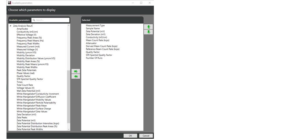
Figure 1: The “Available parameters” list and an example of recommended parameters for interpreting data and results from zeta potential measurement.
Table 2 shows a list of recommended charts that are useful in aiding the interpretation of zeta potential measurements. Charts can be selected from the drop down lists available.
| Chart Name | Description |
|---|---|
| Zeta potential distribution | The zeta potential distribution obtained from the measurement |
| Phase plot | The phase difference between the measured beat frequency and the reference frequency plotted as a function of time |
| Frequency shift | The frequency spectrum obtained from the SFR part of the measurement |
| Zeta potential voltage and current | The voltage and current over the duration of the measurement |
Used in combination, the parameters and charts above allow the user to assess the quality of data and results obtained from zeta potential measurements. To further illustrate this, examples of good and poor data and results will be used.
The repeatability of the zeta potential mean values should be one of the first things to check after measurements have been taken. A number of repeat measurements should be performed on a sample, with a minimum of 3, preferably 5, repeats recommended. A pause between repeat measurements should also be used. The ZS Xplorer software automatically sets a default pause of 60 seconds between repeat measurements to minimize Joule heating and electrode polarization effects.
For a suitable sample, the zeta potential mean values should be within 1 or 2 mV of one another. Values which show trends could be indicative of sample instability or Joule heating/electrode polarization effects. These adverse effects could be minimized by increasing the pause between repeat measurements.
The phase plot chart shows the difference in phase between the measured beat frequency and the reference frequency as a function of time. The Quality Factor is a signal to noise based parameter that is derived from the phase plot data, has a threshold value of 1 and is used to decide when a zeta potential measurement should end if automatic duration is used. Once a value greater than 1 is achieved, the result can be accepted as being reliable.
A typical phase plot of good quality obtained from a measurement using the General Purpose protocol is shown in figure 2. This plot shows well defined, alternating slopes of the phase difference with time, which result from the fast field reversal (FFR) part of the measurement (up to 1.2 seconds). These slopes are averaged to determine the mean phase difference and hence mean zeta potential. In addition, the slopes of the phase difference during the slow field reversal (SFR) part of the measurement are smooth and well defined (between 1.2 and 2.6 seconds). The Quality Factor parameter for this measurement would be greater than 1.
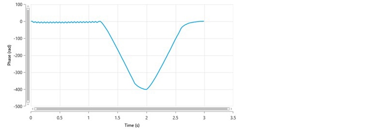
Figure 2: A typical phase plot of good quality from a General Purpose measurement showing the difference in phase between the measured beat frequency and the reference frequency as a function of time.
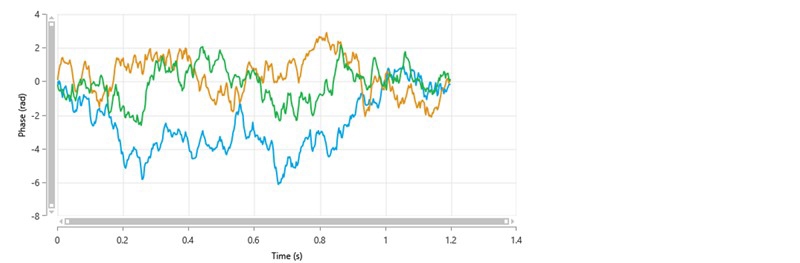
Figure 3 is an example of a poor phase plot obtained from a General Purpose measurement. There are no well-defined alternating slopes during the FFR part of the measurement and the SFR part of the measurement shows noisy data.
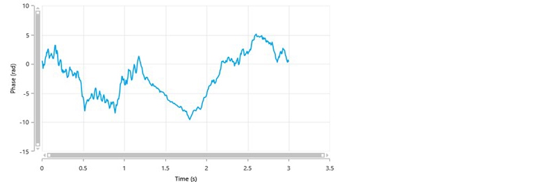
Figure 3: A typical phase plot of poor quality from a General Purpose measurement.
The poor data quality shown may be due to several factors as summarized in Table 3 and further discussed below.
| Reasons for Poor Phase Data | Actions to Improve |
|---|---|
| Sample concentration too low | Increase sample concentration if possible and remeasure |
| Sample concentration too high | Decrease sample concentration if possible and remeasure |
| High conductivity causing sample/electrode degradation/polarization | Ensure that the Monomodal analysis was used |
| Ensure that constant current mode was used | |
| Use diffusion barrier method | |
| Sample has a low or zero zeta potential value | Adjust pH of sample and remeasure to see whether the mean zeta potential value changes |
| Measurement duration manually set | Set measurement duration to automatic and remeasure |
| Measurement of biomolecules such as proteins | Ensure that the Monomodal analysis was used. Use diffusion barrier method and perform size measurements before and after the zeta potential measurements to ensure sample integrity has been maintained |
1. The sample concentration may be too low or too high. The minimum and maximum sample concentrations that can be measured in a Zetasizer Advance instrument will depend on various factors such as the optical properties of the particles, the particle size and the polydispersity of the particle size distribution. The laser beam must penetrate the sample for scattered light at a forward angle to be detected. Therefore, in general, samples for zeta potential measurements must be optically clear. If the concentration of the sample becomes too high, then the laser beam will become attenuated by the particles reducing the scattered light that is detected. If the sample concentration needs to be reduced, the dilution method used should not change the chemistry of the sample. This can be achieved by filtering or centrifuging some clear liquid from the original sample and using this to dilute the original concentrated sample. If a supernatant cannot be extracted, then an alternative is to allow any large particles to naturally sediment and measure the fine particles left in the supernantant. The other method would be to mimic the original medium as close as possible with respect to pH, concentration of each ionic species present and concentration of any additives present.
If the sample concentration is too low, there may be insufficient scattered light being detected. The mean count rate, attenuator and the derived count rate parameters can be used to assess whether the intensity of scattered light detected is appropriate. Measurements of molecular solutions such as proteins can often result in poor phase data due to weak sample scattering. If the sample concentration cannot be increased, the zeta potential mean values should be checked for repeatability to ascertain whether the results are reliable.
Further information on the concentration limits for zeta potential measurements can be found in the Knowledge Center of the Malvern Panalytical website.
The Zetasizer Advance systems contain an automatic attenuator that varies the intensity of the laser beam entering the sample and hence varies the intensity of the scattered light being detected. For samples that do not scatter much light, such as very small particles or samples of low concentration, the amount of scattered light being detected must be increased. The attenuator will therefore automatically allow more light through to the sample. For samples that significantly scatter light, such as large particles or samples at high concentration, the attenuator automatically reduces the amount of light that passes through to the sample. The attenuator in the Zetasizer Advance series has 11 positions covering an attenuator range of 100% to 0.0003%.
A measurement taken with an attenuator position of 11 indicates that the sample concentration may be inappropriate i.e. either too low or too high and may result in poor phase and distribution plots.
Another possibility for low count rates is that either the cell has not been inserted correctly, or there are air bubbles in the path of the laser. If air bubbles are present, the sample should be removed from the cell, re-inserted and re-measured.
2. The second reason for poor phase plot data is that the conductivity of the sample may be high causing sample/electrode degradation if the General Purpose measurement protocol has been used. The application of the field for long periods during the SFR part of the measurement can cause Joule heating, resulting in sample/electrode degradation or a loss of sample integrity. If Auto Mode was used to perform the measurement, the software will optimize the measurement settings from the measured sample conductivity. For example, if the conductivity is <5 mS/cm, 150 V, General Purpose and constant voltage are used. For conductivity values between 5 and 30 mS/cm, 50 V, Monomodal and constant current mode are used. For conductivity values >30 mS/cm, 10 V, Monomodal and constant current mode are used.
If Monomodal is selected, only the FFR part of the measurement is performed and only a mean zeta potential value is obtained i.e. no zeta potential distribution. Figure 4 shows a typical phase plot of good quality obtained from a Monomodal measurement. In this example, the zeta potential of the sample is positive.
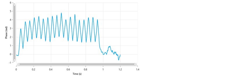
Figure 4: A typical phase plot of good quality from a Monomodal measurement
Zeta potential measurements become more challenging with increasing conductivity due to several factors. These include Joule heating, electrode degradation (blackening), sample degradation (e.g. aggregation/denaturation) and electrode polarization. The automatic settings of the instrument try to minimize these potential problems as much as possible. However, the use of the diffusion barrier method will further help in minimizing any effects of the field on the zeta potential results obtained.
In the diffusion barrier technique, a small plug of sample e.g. 20 μL, is introduced into a folded capillary cell containing the same buffer that the sample is prepared in, and is therefore, isolated from the electrodes. The physical distance between the sample and the electrodes mean that the sample is protected, and its integrity is assured. The diffusion barrier method has the added advantage of requiring smaller sample volumes for measurement and should be used for any sample whose conductivity is greater than 5 mS/cm.
Further information on the diffusion barrier method can be found in the Knowledge Center of the Malvern Panalytical website.
3. The next possible reason for poor phase plot data is that the sample has a low or zero zeta potential value. This will mean that the beat frequency and reference frequency will be the same or very similar and the PALS analysis will result in noisy phase plot data. Adjusting the pH and remeasuring the sample should result in a shift in the mean zeta potential value, confirming that the original sample had a low or zero zeta potential value.
4. Poor phase plot data could be obtained if the measurement duration was manually set to a short time (e.g. 20 sub runs). This can be confirmed by viewing the method of the measurement. The data quality could be improved by using automatic duration and remeasuring the sample.
5. The measurement of biomolecules such as proteins is challenging. Samples are normally prepared at low concentrations in physiological buffers with high conductivities and will be small and weakly scattering which could produce poor phase plot data.
The Monomodal analysis (FFR only) should be used for these types of samples to minimize the application of the applied voltage, electrode polarization and Joule heating effects. It is recommended that the diffusion barrier technique is used, as discussed above, and that size measurements should be performed before and after the zeta potential measurements to check that sample integrity has been maintained. The application of the voltage could lead to denaturation and aggregation of the molecules being measured, resulting in increases in the both the scattering intensities and sizes. Therefore, comparison of the size results after the zeta potential measurements with those obtained before provides confidence in the data.
It is probable that for these types of samples, phase plots will be of poor quality and the Quality Factor parameter may never reach the acceptable threshold value of 1. The repeatability of the zeta potential mean values obtained from several measurements may be compromised. If this is the case, it is does not necessarily mean that the results are not usable. A larger standard deviation across multiple measurements may have to be accepted. As an example, figure 5 shows the phase plots obtained from 3 repeat measurements of a protein solution and table 4 summarizes the zeta potential mean and Quality Factor values.
| Measurement | Zeta Potential Mean (mV) | Quality Factor |
|---|---|---|
| 1 | -4.8 | 0.448 |
| 2 | -2.2 | 0.244 |
| 3 | -4.1 | 0.410 |
| Mean (SD) | -3.7 (1.4) |
None of the Quality Factor values have reached the threshold value of 1. However, the zeta potential mean values show good repeatability, and therefore the results can be considered to be acceptable.
For these types of samples, it is advisable to use a manual duration and reduce the number of sub runs. Minimizing the number of sub runs per measurement should help to minimize electrode polarization and sample degradation.
The zeta potential distribution is derived from the frequency distribution obtained from the SFR part of a General Purpose measurement using a Fourier transform analysis. The SFR Spectral Quality Factor is a signal to noise based parameter derived from the frequency analysis and has a threshold value of 1. Once a value greater than 1 is achieved, the zeta potential distribution can be accepted as being reliable.
The zeta deviation is the standard deviation of the zeta potential distribution and can be used to assess the polydispersity of zeta potentials present in the sample. For example, a bimodal zeta potential distribution will have a larger zeta deviation compared to a monomodal one. A sample which contains very small particles will also display a larger zeta deviation. The smaller the particles/molecules are, the more rapid their Brownian motion becomes causing a broadening of the frequency signal detected, an effect called Brownian broadening.
Occasionally, a zeta potential distribution is obtained which resembles figure 6. In this example, the mean zeta potential value is -21.1 mV and the zeta deviation is 32.5 mV. The most noticeable aspect of this distribution is the presence of peaks both negatively and positively charged, something which is unexpected. The zeta potential peak mean values are -49.0 mV, -28.4 mV and +30.4 mV respectively. The presence of both negative and positive peaks arises because, when the frequency distribution is converted into a zeta potential distribution, the peaks are centered around the mean zeta potential value obtained from the PALS analysis during the FFR part of the measurement. The positive peak present in the distribution is therefore probably an artefact and can be confirmed by looking at the frequency distribution obtained for the measurement.
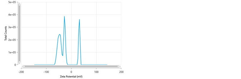
Figure 6: Zeta potential distribution showing the presence of both negatively and positively charged peaks.
The frequency distribution for this result is shown in figure 7. This shows a sharp peak at 1000 Hz which is the reference frequency generated by the modulator. This is indicative of static scattering which can arise due to various reasons such as, a scratch on the folded capillary cell around the measurement zone, air bubbles adsorbed onto the cell wall, finger prints where the laser passes into the cell or adsorbed material on the wall of the cell (for example, this could happen if a cationic sample was being measured as there would be an attraction of the positive particles/molecules to the negatively charged polycarbonate folded capillary cell).
If the cell is found to be scratched, the measurement should be repeated in a new folded capillary cell. Fingerprints or bubbles should be removed, and the measurement repeated.
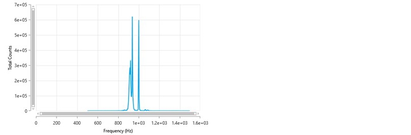
Figure 7: Frequency distribution showing the presence of a sharp peak at 1000 Hz.
This technical note discusses how to interpret zeta potential measurements using various plots and parameters available in the ZS Xplorer software. It should provide guidance of how to assess the quality of data and results obtained and how to improve these if issues are determined.